"Prediction is very difficult, especially if it's about the future."
Social networks are a popular way to model the interactions among the people in a group or community. They can be visualized as graphs, where a vertex corresponds to a person in some group and an edge represents some form of association between the corresponding persons. Social networks are also very dynamic, as new edges and vertices are added to the graph over time. Understanding the dynamics that drive the evolution of a social network is a complex problem due to a large number of variable parameters.
But, a comparatively easier problem is to understand the association between two specific nodes. For instance, some of the interesting questions that can be posed are: How does the association patterns change over time? What are the factors that drive the associations? How is the association between two nodes affected by other nodes? The problem we want to tackle here is to predict the likelihood of a future association between two nodes, knowing that there is no association between the nodes in the current state of the graph. This problem is commonly known as the Link Prediction problem [1].
In effect, the link prediction problem asks: to what extent can the evolution of a social network be modeled using features intrinsic to the network topology itself? Can the current state of the network be used to predict future links?
The link prediction problem is also related to the problem of inferring missing links from an observed network: in a number of domains, one constructs a network of interactions based on observable data and then tries to infer additional links that, while not directly visible, are likely to exist. This line of work differs from our problem formulation in that it works with a static snapshot of a network, rather than considering network evolution; it also tends to take into account specific attributes of the nodes in the network, rather than evaluating the power of prediction methods based purely on the graph structure [2].
For example, in facebook's case, with their "friend finder" feature, they could either suggest people whom you might find interesting enough that the connection may lead to actual friendship in real life (new friend recommender) which could enhance both party's loyalties to facebook's service (thus making facebook more money). Or they could suggest friends you already know, but just not yet connected through facebook (constructing ones current friendship network on facebook). The latter example corresponds to the original problem statemnet while the former example corresponds to the prediction of missing links (second related problem). Alas, facebook only attemps the latter task.
Beyond social networks, link prediction has many other applications. For example, in bioinformatics, link prediction can be used to find interactions between proteins [Airoldi et al. 2006]; in e-commerce it can help build recommendation systems [Huang et al. 2005] such as the "people who bought this also bought" feature on Amazon; and in the security domain link prediction can assist in identifying hidden groups of terrorists or criminals [Hasan et al. 2006]. In addition, many studies have been carried out on co-authorship networks (for example in scientific journals, with edges joining pairs who have co-authored papers). Two scientists who are “close” in the network will have colleagues in common and will travel in similar circles; this social proximity suggesting that they themselves are more likely to collaborate in the near future. Thus link prediction in this application could be used to accelerate a mutually beneficial professional or academic connection/collaborations that would have taken longer to form serendipitously.
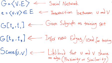
We are given an unweighted, undirected graph G = ⟨V,E⟩ representing the topological structure of a social network in which each
edge e = ⟨u,v⟩ ∈ E represents an interaction between u and v that took place at a particular time t(e). For two times t and t′ > t, let G[t,t′] denote the subgraph of G consisting of all edges with a timestamp between t and t′. Let t0, t′0, t1, and t′1 be four times, where t0 < t′0 ≤ t1 < t′1. Then the link prediction task is: given network G[t0, t′0]; output a list of edges not present in G[t0, t′0] that are predicted to appear in the network G[t1,t′1]. We refer to [t0,t′0] as the training interval and [t1, t′1] as the test interval.
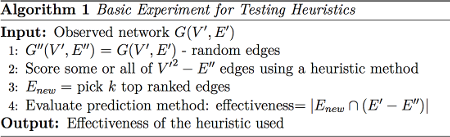
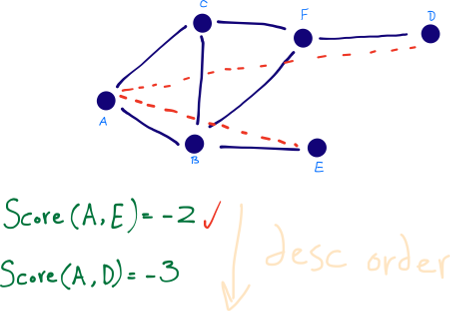
To generate this list, we use heuristic algorithms which assign a similarity matrix S whose real entry sxy is the score between x and y. This score can be viewed as a measure of similarity between nodes x and y. For each pair of nodes, x, y ∈ V, generally sxy = syx. All the nonexistent links are sorted in decreasing order according to their scores, and the links at the top are most likely to exist [4].
Since we can't actually predict the future, to test the algorithm’s accuracy, a fraction of the observed links E (lets say 90% of the whole) of some known interaction dataset is randomly singled out as a training set, ET, the remaining links (10% of the whole) are used as the probe set, EP, to be predicted and no information in this set is allowed to be used for prediction. Clearly, E=ET ∪ EP and ET ∩ EP=ø. The prediction quality is evaluated by a standard metric, the area under the receiver operating characteristic curve (AUC). This metric can be interpreted as the probability that randomly chosen missing link (a link in EP) is given a higher score than a randomly chosen nonexistent link (a link in U but not in E, where U denotes the universal set)[8]. Among n independent comparisons, if there are n′ occurrences of missing links having a higher score and n′′ occurrences of missing links and nonexistent link having the same score, we define the accuracy as:
AUC = (n′ + 0.5n′′) / n
If all the scores are generated from an independent and identical distribution, the accuracy should be about 0.5. Therefore, the degree to which the accuracy exceeds 0.5 indicates how much better the algorithm performs than pure chance.
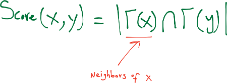
 Also, for a node x, Γ(x) represents the set of neighbors of x. degree(x) is the size of the Γ(x).
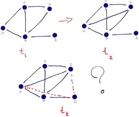 Given a snapshot of a social network at time t (or network evolution between t1 and t2), we seek to accurately predict the edges that will be added to the network during the interval from time t (or t2) to a given future time t'.
Social networks are defined by structures whose nodes represent people or other entities embedded in a social context, and whose edges represent interaction, collaboration, or influence between entities. As such, these networks have several well-known characteristics, such as the power law degree distribution [Barabasi and Albert 1999], the small world phenomenon [Watts and Strogatz 1998], and the community structure (clustering effect) [Girvan and Newman 2002].
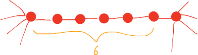
The small world effect refers to the phenomenon that the average distance in the network is very small compared to the size of the network. That is to say, each pair of nodes can be connected through a short path in a network. In his famous experiments, Stanley Milgram challenged people to route postcards to a fixed recipient by passing them only through direct acquaintances. Milgram found that the average number of intermediaries on the path of the postcards lay between 4.4 and 5.7, depending on the sample of people chosen. Facebook just recently reported the results of their first world-scale social-network graph-distance computation, using the entire Facebook network of active users (721 million users, 69 billion friendship links). They found that the average distance was 4.74, corresponding to 3.74 intermediaries or “degrees of separation”.
The scale-free effect refers to the phenomenon that most nodes’ links are very small in the network; only a few nodes have lots of links. In such network, nodes with high degree are called hubs (hinge node). The hub node dominates the network operation. Scale-free effect shows that node degree distribution is seriously uneven in large-scale network. areto, heavy-tailed, or Zipfian degree distributions.) This phenomenon was noted for the degree distribution of the world-wide web
The clustering effect refers to the phenomenon that there is a circle of friends, acquaintances, rings, and other small groups in social network. Each member of the small group knows each other. This phenomenon can also be described by the concept of triadic closure: that there is many fully connected subgraphs in social network.
For a social network G(V,E), there are V × V – E possible edges to choose from, if we were picking a random edge to predict for our existing social network. If G is dense, then E ≈ V2 - b where b is some constant between 1 and V. Thus, we have a constant number of edges to choose from, and O(1/c) probability of choosing correctly at random. If G is sparse, then E ≈ V. Thus, we have a V2 edges to choose from, and O(1/V2) probability of choosing correctly at random. Unfortunately social networks are sparse, so picking at random is a terrible idea!
In the DBLP dataset, in the year 2000, the ratio of actual and possible link is as low as 2 × 10⁻⁵. So, in a uniformly sampled dataset with one million training instances, we can expect only 20 positive instances. Even worse, the ratio between the number of positive links and the number of possible links also slowly decreases over time, since the negative links grow quadratically whereas positive links grow only linearly with a new node.
For a period of 10 years, from 1995 to 2004 the number of authors in DBLP increased from 22 thousand to 286 thousand, meaning the possible collaborations increased by a factor of 169, whereas the actual collaborations increased by only a factor of 21.
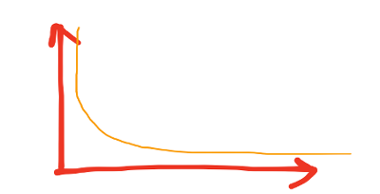
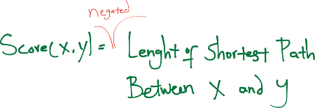
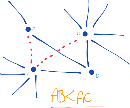
Graph Distance Perhaps the most direct metric for quantifying how close two nodes are is the graph distance. It is defined as the negative of the shortest-path distance from x to y.
Note that it is inefficient to apply Dijkstra’s algorithm to compute shortest path distance from x to y when G has millions of nodes. Instead, we exploit the small-world property of the social network and apply expanded ring search to compute the shortest path distance from x to y.
Specifically, we initialize S = {x} and D = {y}. In each step we either expand set S to include its members’ neighbors (i.e., S = S ∪ {v|⟨u, v⟩ ∈ E ∧ u ∈ S}) or expand set D to include its members’ inverse neighbors (i.e., D = D ∪ {u|⟨u, v⟩ ∈ E ∧ v ∈ D}). We stop whenever S ∩ D != ∅ . The number of steps taken so far gives the shortest path distance. For efficiency, we always expand the smaller set between S and D in each step. [10]
Common Neighbors The common-neighbors predictor captures the notion that two strangers who have a common friend may be introduced by that friend. This introduction has the effect of “closing a triangle” in the graph and feels like a common mechanism in real life. Newman [7] has computed this quantity in the context of collaboration networks, verifying a positive correlation between the number of common neighbors of x and y at time t, and the probability that x and y will collaborate at some time after t.
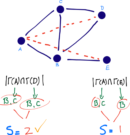
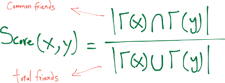
Jaccard’s Coefficient The Jaccard coefficient—a similarity metric that is commonly used in information retrieval— measures the probability that both x and y have a feature f, for a randomly selected feature f that either x or y has. If we take “features” here to be neighbors, then this measure captures the intuitively appealing notion that the proportion of the coauthors of x who have also worked with y (and vice versa) is a good measure of the similarity of x and y.
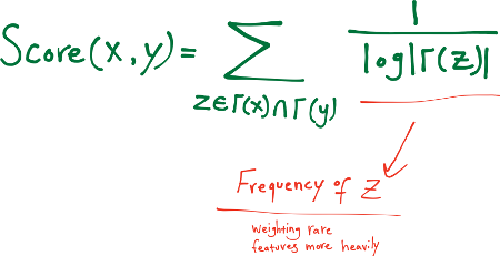
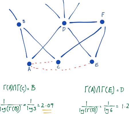
Adamic/Adar (Frequency-Weighted Common Neighbors) This measure refines the simple counting of common features by weighting rarer features more heavily. The Adamic/Adar predictor formalizes the intuitive notion that rare features are more telling; documents that share the phrase “for example” are probably less similar than documents that share the phrase “clustering coefficient.”
If “triangle closing” is a frequent mechanism by which
new edges form in a social network, then for x and y to be introduced by a common friend z,
person z will have to choose to introduce the pair ⟨x,y⟩ from
(choose |Γ(z)| with 2) pairs of his friends; thus
an unpopular person (someone with not a lot of friends) may be more likely to introduce a particular pair of his friends to each other.
Preferential Attachment One well-known concept in social networks is that users with many friends tend to create more connections in the future. This is due to the fact that in some social networks, like in finance, the rich get richer. We estimate how ”rich” our two vertices are by calculating the multiplication between the number of friends (|Γ(x)|) or followers each vertex has. It may be noted that the similarity index does not require any node neighbor information; therefore, this similarity index has the lowest computational complexity.

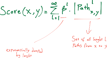
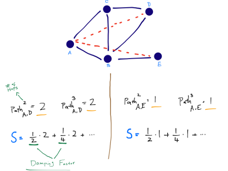
Katz (Exponentially Damped Path Counts) This heuristic defines a measure that directly sums over collection of paths, exponentially damped by length to count short paths more heavily. The Katz-measure is a variant of the shortest-path measure. The idea behind the Katz-measure is that the more paths there are between two vertices and the shorter these paths are, the stronger the connection.
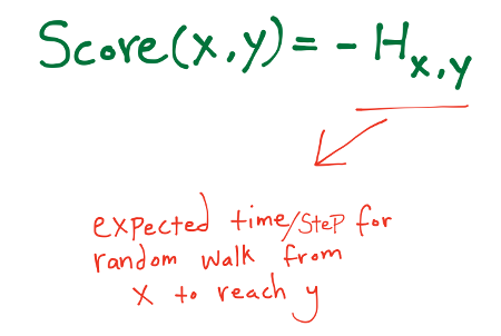
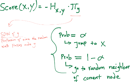
Hitting Time A random walk starts at a node x and iteratively moves to a neighbor of x chosen uniformly at random. The hitting time Hx,y from x to y is the expected number of steps required for a random walk starting at x to reach y.
One difficulty with hitting time as a measure of proximity is that Hx,y is quite small whenever y is a node with a large stationary probability πy, regardless of the identity of x (That is, for a node y at which the random walk spends a considerable amount of time in the limit, the random walk will soon arrive at y, almost no matter where it starts. Thus the predictions made based upon Hx,y tend to include only a few distinct nodes y) To counter-balance this phenomenon, we also consider normalized versions of the hitting and commute times, by defining
score(x, y) = −Hx,y · πy
Rooted PageRank Another difficulty with using the measures based on hitting time and commute time is their sensitive dependence to parts of the graph far away from x and y, even when x and y are connected by very short paths. A way of counteracting this difficulty is to allow the random walk from x to y to periodically “reset,” returning to x with a fixed probability α at each step; in this way, distant parts of the graph will almost never be explored.
Random resets form the basis of the PageRank measure for web pages, and we can adapt it for link prediction. Similar approaches have been considered for personalized PageRank, in which one wishes to rank web pages based both on overall “importance” (the core of PageRank) and relevance to a particular topic or individual, by biasing the random resets towards topically relevant or bookmarked pages
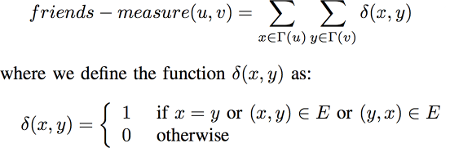
Other metrics Another metric that can be used is the Friends-measure. When looking at two vertices in a social network, we can assume that the more connections their neighborhoods have with each other, the higher the chances the two vertices are connected. We take the logic of this statement and define the Friends-measure as the number of connections between u and v neighborhoods. One can notice that in undirected networks, the Friends-measure is a private case of the Katz-measure where β = 1 and lmax = 2.
Generally, the link prediction algorithms based on network topologies are designed according to the measures of the structural similarity of nodes, which can be classified as local and global methods. Overall they can be classified as such:
Among these, node-neighborhood-based algorithms have restricted scalability, and do not necessarily constitute a viable approach for User Generated Content networks [9]. For example, Facebook has more than one billion registered users and each month many new users are added. Moreover, the power law degree distribution in social networks suggests that there are some individuals with a large number of connections (hubs). Computing local topological features on a subgraph consisting only of the friends of these individuals may be computationally intensive.
On the right are the performance charts calculated by Liben-Nowell and Kleinberg in 2003, who studied the usefulness of graph topological features by testing them on five co-authorship network datasets, each containing several thousands of authors [3].
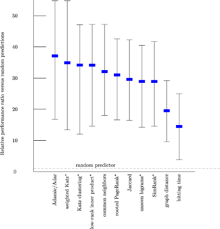 The number on the left is the number of factor of improvements over the random prediction. i.e. the Adamic/Adar mesure is about 37 times more accurate than the random predictor
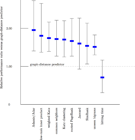 Comparison with the graph distance predictor as the baseline. The improvements suddenyl don't seem very impressive.
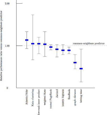 Comparison with the common neighbor predictor as the baseline. The other measure are now only marginally better!
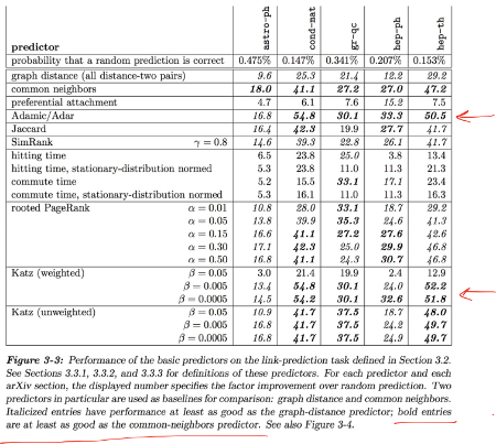 Chart showing the numerical results on multiple sections of the arVix coauthorship network. Different sections of arXiv yield different results.
Although features intrinsic to a network can offer a good measure of how likely a future link is (can significantly outperform chance), many other metrics/methods have also been proposed which are usually a variation of the heuristics mentioned. For example, Extra-network features can significantly improve prediction accuracy (i.e. keywords describing interests of each scientist, or keywords extracted from their papers/abstracts/titles).
Or considering the time characteristics of the network, social network graph can be divided into different graph sequences in accordance with a certain time step. The moving average is the average of an heuristics value for an edge in a certain period time [13]. By looking at this average over many generations of evolution, one can make very accurate link predictions.
Moreover, link prediction problem is studied in the supervised learning framework by treating it as an instance of binary classification These methods use the topological and semantic measures defined between nodes as features for learning classifiers. Given a snapshot of the social network at time t for training, they consider all the links present at time t as positive examples and consider a large sample of absent links (pair of nodes which are not connected) at time t as negative examples. The learned classifiers performed consistently across all the datasets unlike heuristic methods which were inconsistent, although the accuracy of prediction is still very low [14].
There are several reasons for this low prediction accuracy. One of the main reasons is the huge class skew associated with link prediction. In large networks, it’s not uncommon for the prior link probability on the order of 10^−4 or less, which makes the prediction problem very hard, resulting in poor performance. In addition, as networks evolve over time, the negative links grow quadratically whereas positive links grow only linearly with new nodes.
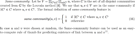 The same community metric calculates the intuition that people who belong to the same community will probably be linked.
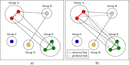 Actors in the same tightly-knit group often exhibit structural equivalence, i.e., they have the same
connections to all other nodes. Using the original network (a), and a structural equivalence assumption, one
can construct a network with new predicted links (b).[11]
Actors in the same tightly-knit group often exhibit structural equivalence, i.e., they have the same
connections to all other nodes. Using the original network (a), and a structural equivalence assumption, one
can construct a network with new predicted links (b).[11]
This page was created as a class project for COMP 260: Advanced Algorithms (Spring 2014). I've made a pdf presentation (in the style of class presentations) for this project as well.
Thanks to Professor Aloupis and to Andrew Winslow for a great class and semester. Lastly, the page design is from Bret Vistor's WorryDream.